T2: Downstream Proteomics

Analyzing downstream proteomics is fun!
In this tutorial we will show you how to take a quick look at your data, check the proteomic distributions.
Filter the dataset to remove low quality proteins, and impute the data for dimensionality reduction.
Then we perform some simple statistical test and plot it with the famous volcano plot.

Introduction

Package import

import opendvp as dvp
import pandas as pd
import numpy as np
import scanpy as sc

import seaborn as sns
import matplotlib.pyplot as plt

print(f"openDVP version {dvp.__version__}")

openDVP version 0.6.4

Load DIANN data into an adata object

Mass spectrometers produce spectra of your protein fragments.
These peaks needs to be mapped to peptides from a database, and then infer the present proteins.

We use DIANN, a software tool used to streamline this process and obtain a relative quantfication of our proteins.
We now use one of the DIANN outputs, the protein group matrix (pg_matrix), to perform downstream analysis.

Therefore, our first step is to convert DIANN to adata.

adata = dvp.io.DIANN_to_adata(
    DIANN_path="../data/proteomics/DIANN_pg_matrix.csv",
    DIANN_sep="\t",
    metadata_path="../data/proteomics/DIANN_metadata.csv",
    metadata_sep=";",
    n_of_protein_metadata_cols=4,
)

16:49:01.64 | INFO | Starting DIANN matrix shape (7030, 14)
16:49:01.64 | INFO | Removing 264 contaminants
16:49:01.65 | INFO | Filtering 3 genes that are NaN
16:49:01.65 | INFO | ['A0A0G2JRQ6_HUMAN', 'A0A0J9YY99_HUMAN', 'YJ005_HUMAN']
16:49:01.66 | INFO | 10 samples, and 6763 proteins
16:49:01.67 | INFO | 52 gene lists (eg 'TMA7;TMA7B') were simplified to ('TMA7').
16:49:01.67 | SUCCESS | Anndata object has been created :)

This function performs of helpful functionalities under the hood:

1. It removes known contaminants from your samples.

2. It removes any protein groups that do not have a valid gene name (NaN)

3. Gene strings like 'TMA7;TMA7B' are simplified to TMA7 for streamlining with other tools.

Quick look at adata object

adata

AnnData object with n_obs × n_vars = 10 × 6763
    obs: 'Precursors.Identified', 'Proteins.Identified', 'Average.Missed.Tryptic.Cleavages', 'LCMS_run_id', 'RCN', 'RCN_long', 'QuPath_class'
    var: 'Protein.Group', 'Protein.Names', 'Genes', 'First.Protein.Description'

# Quantification values, we can see missing values already :)
adata.X[:5, :5]

array([[     nan,  5387.49, 10755.7 , 21750.3 , 20374.3 ],
       [ 9623.48,      nan,      nan,  8450.09,      nan],
       [ 8161.97,      nan,      nan, 14534.7 , 16192.5 ],
       [ 7438.25,      nan,      nan,  7547.04, 13379.7 ],
       [     nan,      nan,  9925.7 , 19308.4 , 16956.7 ]])

# Variable metadata, in this case proteins/genes
adata.var.head()

	Protein.Group	Protein.Names	Genes	First.Protein.Description
Gene
TMA7	A0A024R1R8;Q9Y2S6	TMA7B_HUMAN;TMA7_HUMAN	TMA7;TMA7B	Translation machinery-associated protein 7B
IGLV8-61	A0A075B6I0	LV861_HUMAN	IGLV8-61	Immunoglobulin lambda variable 8-61
IGLV3-10	A0A075B6K4	LV310_HUMAN	IGLV3-10	Immunoglobulin lambda variable 3-10
IGLV3-9	A0A075B6K5	LV39_HUMAN	IGLV3-9	Immunoglobulin lambda variable 3-9
IGKV2-28	A0A075B6P5;P01615	KV228_HUMAN;KVD28_HUMAN	IGKV2-28;IGKV2D-28	Immunoglobulin kappa variable 2-28

# Observations metadata, in this case each proteomic sample
adata.obs.head()

	Precursors.Identified	Proteins.Identified	Average.Missed.Tryptic.Cleavages	LCMS_run_id	RCN	RCN_long	QuPath_class
Sample_filepath
Sample_1	26358	4760	0.139	8674	RCN1	Tumor enriched	P12_Tumor_1
Sample_2	24705	4553	0.134	8452	RCN1	Tumor enriched	P12_Tumor_2
Sample_3	26750	4835	0.134	8414	RCN1	Tumor enriched	P12_Tumor_3
Sample_4	24268	4502	0.116	8551	RCN1	Tumor enriched	P12_Tumor_4
Sample_5	27883	4858	0.136	8424	RCN1	Tumor enriched	P12_Tumor_5

Describing the dataset

This dataset is a subset of the Triple Negative Breast Cancer dataset investigated in the openDVP paper.
Briefly, we performed image analysis, and based on the recurrent cellular neighborhoods(RCN) we performed our laser microddisection.
We collected samples from tumor enriched areas and immune enriched areas.
Here we explore how their proteomes differ.

adata.obs.columns

Index(['Precursors.Identified', 'Proteins.Identified',
       'Average.Missed.Tryptic.Cleavages', 'LCMS_run_id', 'RCN', 'RCN_long',
       'QuPath_class'],
      dtype='object')

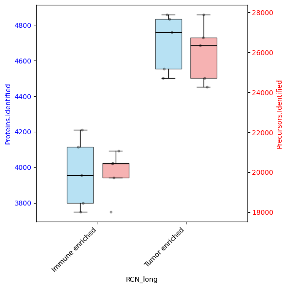
# Let's see how many proteins and precursors were measured per sample
dvp.plotting.dual_axis_boxplots(
    adata=adata, feature_1="Proteins.Identified", feature_2="Precursors.Identified", group_by="RCN_long"
)

Exploring the protein quantification

Modern mass spectrometry workflows have a dynamic range of 5 to 6 orders of magnitude.
To have a more statistically normal distribution, and have a more intuitive range of data, we use log2 transformation.

print(f"Maximum value: {np.nanmax(adata.X)}")
print(f"Minimum value: {np.nanmin(adata.X)}")

Maximum value: 11506600.0
Minimum value: 251.795

# Log2 transform the data
adata.X = np.log2(adata.X)

print(f"Maximum value: {np.nanmax(adata.X)}")
print(f"Minimum value: {np.nanmin(adata.X)}")

Maximum value: 23.45595826937909
Minimum value: 7.976105824909396

fig, axes = plt.subplots(nrows=1, ncols=2, figsize=(10, 5))
dvp.plotting.density(adata=adata, color_by="RCN_long", ax=axes[0])
dvp.plotting.density(adata=adata, color_by="QuPath_class", ax=axes[1])
plt.show()

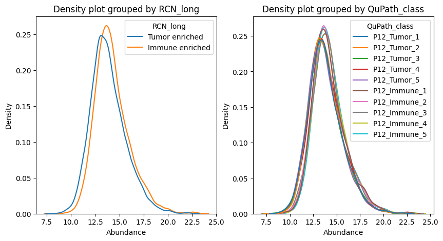
These density graphs already show us little difference between samples, in terms of overall quantifications.

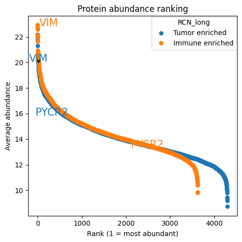
dvp.plotting.rankplot(
    adata=adata, adata_obs_key="RCN_long", min_presence_fraction=0.7, proteins_to_label=["VIM", "PYCR2"]
)

16:50:41.85 | INFO | no groups passed, using ['Tumor enriched', 'Immune enriched']

Preprocess dataset

Filter dataset by NaNs

We expect a lot of proteins to be removed because this is a subsampled dataset.
Many protein hits were present in other groups not present here.

adata_filtered = dvp.tl.filter_features_byNaNs(adata=adata, threshold=0.7, grouping="RCN")

16:50:52.54 | INFO | Filtering protein with at least 70.0% valid values in ANY group
16:50:52.54 | INFO | Calculating overall QC metrics for all features.
16:50:52.54 | INFO | Filtering by groups, RCN: ['RCN1', 'RCN3']
16:50:52.54 | INFO |  RCN1 has 5 samples
16:50:52.55 | INFO |  RCN3 has 5 samples
16:50:52.55 | INFO | Keeping proteins that pass 'ANY' group criteria.
16:50:52.55 | INFO | Complete QC metrics for all initial features stored in `adata.uns['filter_features_byNaNs_qc_metrics']`.
16:50:52.56 | INFO | 4637 proteins were kept.
16:50:52.56 | INFO | 2126 proteins were removed.
16:50:52.57 | SUCCESS | filter_features_byNaNs complete.

adata_filtered.uns["filter_features_byNaNs_qc_metrics"].head()

	Protein.Group	Protein.Names	Genes	First.Protein.Description	overall_mean	overall_nan_count	overall_valid_count	overall_nan_proportions	overall_valid	RCN1_mean	...	RCN1_nan_proportions	RCN1_valid	RCN3_mean	RCN3_nan_count	RCN3_valid_count	RCN3_nan_proportions	RCN3_valid	valid_in_all_groups	valid_in_any_group	not_valid_in_any_group
Gene
TMA7	A0A024R1R8;Q9Y2S6	TMA7B_HUMAN;TMA7_HUMAN	TMA7;TMA7B	Translation machinery-associated protein 7B	13.391	5	5	0.5	False	13.029	...	0.4	False	13.933	3	2	0.6	False	False	False	True
IGLV8-61	A0A075B6I0	LV861_HUMAN	IGLV8-61	Immunoglobulin lambda variable 8-61	13.666	6	4	0.6	False	12.395	...	0.8	False	14.090	2	3	0.4	False	False	False	True
IGLV3-10	A0A075B6K4	LV310_HUMAN	IGLV3-10	Immunoglobulin lambda variable 3-10	14.216	6	4	0.6	False	13.335	...	0.6	False	15.097	3	2	0.6	False	False	False	True
IGLV3-9	A0A075B6K5	LV39_HUMAN	IGLV3-9	Immunoglobulin lambda variable 3-9	15.293	0	10	0.0	True	13.680	...	0.0	True	16.906	0	5	0.0	True	True	True	False
IGKV2-28	A0A075B6P5;P01615	KV228_HUMAN;KVD28_HUMAN	IGKV2-28;IGKV2D-28	Immunoglobulin kappa variable 2-28	15.343	1	9	0.1	True	14.014	...	0.2	True	16.407	0	5	0.0	True	True	True	False

5 rows × 22 columns

adata_filtered.uns["filter_features_byNaNs_qc_metrics"].columns

Index(['Protein.Group', 'Protein.Names', 'Genes', 'First.Protein.Description',
       'overall_mean', 'overall_nan_count', 'overall_valid_count',
       'overall_nan_proportions', 'overall_valid', 'RCN1_mean',
       'RCN1_nan_count', 'RCN1_valid_count', 'RCN1_nan_proportions',
       'RCN1_valid', 'RCN3_mean', 'RCN3_nan_count', 'RCN3_valid_count',
       'RCN3_nan_proportions', 'RCN3_valid', 'valid_in_all_groups',
       'valid_in_any_group', 'not_valid_in_any_group'],
      dtype='object')

In this dataframe, stored away in adata.uns, you can see all th qc metrics of the filtering

# Store filtered adata
dvp.io.export_adata(adata=adata_filtered, path_to_dir="../data/checkpoints", checkpoint_name="2_filtered")

16:50:58.34 | INFO | Writing h5ad
16:50:58.40 | SUCCESS | Wrote h5ad file

Imputation

adata_imputed = dvp.tl.impute_gaussian(adata=adata_filtered, mean_shift=-1.8, std_dev_shift=0.3)

16:51:00.54 | INFO | Storing original data in `adata.layers['unimputed']`.
16:51:00.54 | INFO | Imputation with Gaussian distribution PER PROTEIN
16:51:00.55 | INFO | Mean number of missing values per sample: 572.6 out of 4637 proteins
16:51:00.55 | INFO | Mean number of missing values per protein: 1.23 out of 10 samples
16:51:02.21 | INFO | Imputation complete. QC metrics stored in `adata.uns['impute_gaussian_qc_metrics']`.

adata_imputed

AnnData object with n_obs × n_vars = 10 × 4637
    obs: 'Precursors.Identified', 'Proteins.Identified', 'Average.Missed.Tryptic.Cleavages', 'LCMS_run_id', 'RCN', 'RCN_long', 'QuPath_class'
    var: 'Protein.Group', 'Protein.Names', 'Genes', 'First.Protein.Description', 'mean', 'nan_proportions'
    uns: 'filter_features_byNaNs_qc_metrics', 'impute_gaussian_qc_metrics'
    layers: 'unimputed'

Like the previous process, the imputation stores two quality control datasets.
First, the impute_gaussian_qc_metrics Showing you per protein:

• how many values were imputed

• the distribution used

• the values used to impute with

adata_imputed.uns["impute_gaussian_qc_metrics"]

	n_imputed	imputation_mean	imputation_stddev	imputed_values
Gene
IGLV3-9	0	15.292778	1.840310	NAN
IGKV2-28	1	15.343103	1.346909	[13.0819]
IGHV3-64	6	13.710045	1.247562	[11.7351, 11.3062, 11.8148, 11.6849, 12.0622, ...
IGKV2D-29	0	16.213394	1.481762	NAN
IGKV1-27	0	13.452261	1.394043	NAN
...	...	...	...	...
WASF2	0	15.135411	0.255652	NAN
MAU2	1	12.475482	0.455856	[11.6512]
ENPP4	0	12.008373	0.630813	NAN
MORC2	1	12.330734	0.783775	[10.7016]
SEC23IP	0	14.050191	0.227216	NAN

4637 rows × 4 columns

Second, the unimputed values are stored inside the layers compartment of the adata object.
This is a backup in case imputation has done something wrong.
You can always call those values by adata_imputed.layers['unimputed']

dvp.io.export_adata(adata=adata_imputed, path_to_dir="../data/checkpoints", checkpoint_name="3_imputed")

16:51:10.48 | INFO | Writing h5ad
16:51:10.54 | SUCCESS | Wrote h5ad file

Let’s start with the biology

PCA (courtesy of Scanpy)

sc.pp.pca(adata_imputed)

Scanpy is a very powerful data analysis package created for single-cell RNA sequencing.
We use it here because it is very convenient, and it already expects the AnnData format we have.
Beware of using Scanpy for proteomics datasets, assumptions will vary.

adata_imputed

AnnData object with n_obs × n_vars = 10 × 4637
    obs: 'Precursors.Identified', 'Proteins.Identified', 'Average.Missed.Tryptic.Cleavages', 'LCMS_run_id', 'RCN', 'RCN_long', 'QuPath_class'
    var: 'Protein.Group', 'Protein.Names', 'Genes', 'First.Protein.Description', 'mean', 'nan_proportions'
    uns: 'filter_features_byNaNs_qc_metrics', 'impute_gaussian_qc_metrics', 'pca'
    obsm: 'X_pca'
    varm: 'PCs'
    layers: 'unimputed'

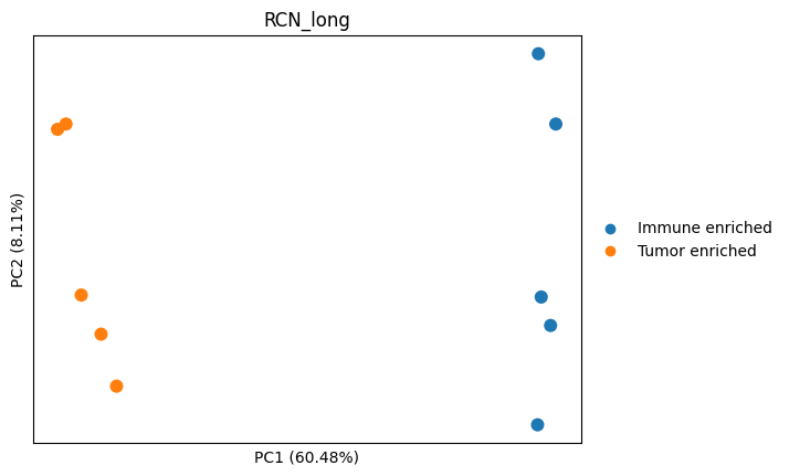
# let's plot it
sc.pl.pca(adata_imputed, color="RCN_long", annotate_var_explained=True, size=300)

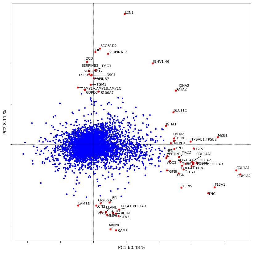
# let's plot the contribution of each protein to the PC1 and PC2
dvp.plotting.pca_loadings(adata_imputed)

19 [ 0.54586545 -0.69229984]
58 [0.65783205 0.95656296]

dvp.io.export_adata(adata=adata_imputed, path_to_dir="../data/checkpoints", checkpoint_name="4_pca")

16:51:23.73 | INFO | Writing h5ad
16:51:23.78 | SUCCESS | Wrote h5ad file

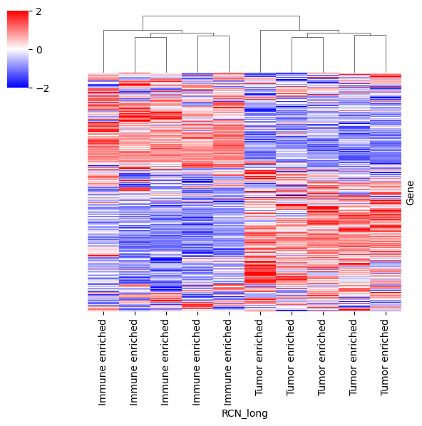
Protein intensities to find patterns at high level

dataframe = pd.DataFrame(data=adata_imputed.X, columns=adata_imputed.var_names, index=adata_imputed.obs.RCN_long)

cm = sns.clustermap(data=dataframe.T, z_score=0, cmap="bwr", vmin=-2, vmax=2, yticklabels=False, figsize=(6, 6))

# to hide dendrogram of proteins
cm.ax_row_dendrogram.set_visible(False)

Differential analysis

# ttest
adata_DAP = dvp.tl.stats_ttest(
    adata_imputed, grouping="RCN_long", group1="Tumor enriched", group2="Immune enriched", FDR_threshold=0.05
)

16:51:35.87 | INFO | Using pingouin.ttest to perform unpaired two-sided t-test between Tumor enriched and Immune enriched
16:51:35.87 | INFO | Using Benjamini-Hochberg for FDR correction, with a threshold of 0.05
16:51:35.87 | INFO | The test found 2003 proteins to be significantly

adata_DAP

AnnData object with n_obs × n_vars = 10 × 4637
    obs: 'Precursors.Identified', 'Proteins.Identified', 'Average.Missed.Tryptic.Cleavages', 'LCMS_run_id', 'RCN', 'RCN_long', 'QuPath_class'
    var: 'Protein.Group', 'Protein.Names', 'Genes', 'First.Protein.Description', 'mean', 'nan_proportions', 't_val', 'p_val', 'mean_diff', 'sig', 'p_corr', '-log10_p_corr'
    uns: 'filter_features_byNaNs_qc_metrics', 'impute_gaussian_qc_metrics', 'pca', 'RCN_long_colors'
    obsm: 'X_pca'
    varm: 'PCs'
    layers: 'unimputed'

dvp.io.export_adata(adata=adata_DAP, path_to_dir="../data/checkpoints", checkpoint_name="5_DAP")

16:51:39.99 | INFO | Writing h5ad
16:51:40.04 | SUCCESS | Wrote h5ad file

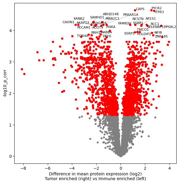
Volcano plot

fig, ax = plt.subplots(figsize=(7, 7))
dvp.plotting.volcano(
    adata=adata_DAP,
    x="mean_diff",
    y="-log10_p_corr",
    FDR=0.05,
    significant=True,
    tag_top=30,
    group1="Tumor enriched",
    group2="Immune enriched",
    ax=ax,
)